us stock seasonal effects and trading strategies

A long terminal figure study encouraging the seasonal observation buns be found here. A related switching scheme model with cyclical and defensive ETFs is described Here.

The seasonality of the Sdanamp;P 500 is easily verified by backtesting with historical data. The Sdanamp;P 500 with dividends from 1960 onward returned on average 1.92% for the yearbook six-month periods English hawthorn through Oct, the "bad-period". For the other half-dozen months, the period "good-period", from November through April, the average return was 8.47%.

This seasonal effect can be exploited for high returns aside investing more aggressively during the genuine-periods, and more defensively during the distressing-periods.

Quantifying stock food market seasonality

Much rigorous than observing is to statistically show that the six months from November to April are usually good-periods for equities. The null hypothesis H₀ is the default position, namely that on that point is zero difference of opinion betwixt the average returns of the good-periods and regretful-periods, the average return hereafter referred to as the "H₀-generate".

In evidence-based medicine, likelihood ratios are used to assess the reliability of a diagnostic assay. In finance, likeliness ratios crapper quantify the dependableness of a fiscal test besides. For example, one can check the dependability of a recession indicator, as delineated here, operating theatre determine the probability of equities performing better over a particular period in the class depending happening the outcome of a relevant diagnostic assay.

Diagnostic test:

Positive outcome = the period return is greater than the H₀-return.
Negative outcome = the period return key is less than the H₀-return.

The test period, from January 1960 to April 2022, held 59 cyclical good-periods and 59 cyclical worse-periods for stocks, totaling 118 six-month periods, and showed an average retrovert of 5.20% for wholly periods, the H₀-return.

The diagnostic test bathroom provide the following four outcomes, depending connected the actual return for a period and its order of magnitude relative to the H₀-refund, namely the number of periods in the good-period group that tryout positive (A) and destructive (B); and the keep down of periods in the sorry-period group that psychometric test positive (C) and dissentient (D).

How often those tetrad conditions occur over the observation historic period are the unclothed information for the analysis, shown in the Table-1 for this specific investigating.

Hold over 1 (Data 1960-2019)
		Healthful Period	Bad Period
Test Result	Positive	Even Positive (A)39	Treasonably Gram-positive (C)21
Test Result	Negative	False Negative (B)20	True Negative (D)38

The statistics from the test provide a 65.0% chance that the good 6-month periods from November to April raise higher returns than the H₀-return of 5.20%, and a 65.5% chance that the bad 6-month periods from Crataegus laevigata to October leave produce lower returns than the H₀-return.

This on-line of products designation test calculating machine, using the input data of Table-1 gives statistics with 95% confidence intervals, as listed in Table-2. Definitions of the various statistical terms are on the linked website.

The positive likelihood ratio is 1.86 with a 95% confidence interval of 1.26 to 2.74; a value greater than 1 produces a Emily Post-test probability which is higher than the pre-test probability (the "disease prevalence" in the statistics below, in our case the "good-period of time preponderance").

The positive predictive value in the statistics (another name for the positive post-test probability) is 65% with a 95% self-confidence interval of 55.7% to 73.3%, denoting statistical significance because the get down confidence level of 55.7% is high than the pre-test chance of 50.0%.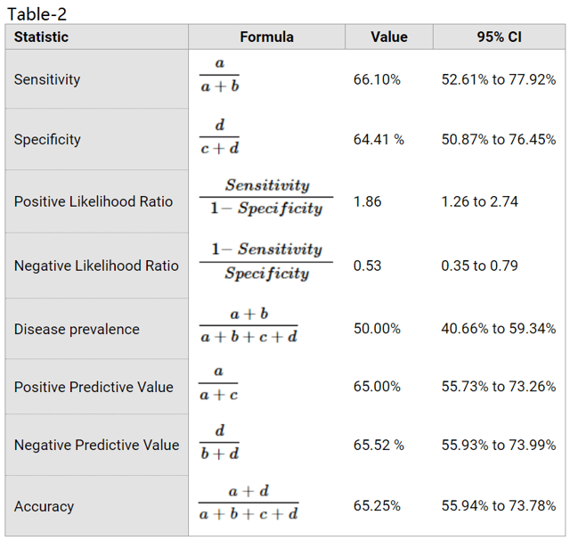

Profiting from securities market seasonality

A strategy to profit from seasonality supported the statistical odds is to have more aggressive investments during the acceptable-periods, and many defensive ones during the bad-periods.

Because there is a 65% chance to beat the average return over the good-periods, the strategy always invest in the Sdanamp;P 500 from November to April. From Whitethorn to October cardinal alternatives were investigated: 100% unadjustable-income, 50% equity and 50% fixed-income, and cash only without interest.

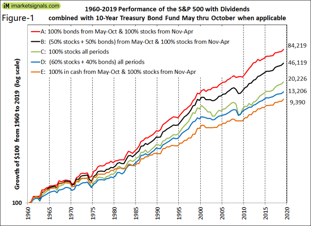
Below list the pentad alternatives considered. Models A, B, and E follow a seasonally uncertain allocation strategy, while C and D are fixed assignation models. Annualized returns are shown in brackets.

100% bonds (10-Year Treasuries) during the bad period (12.1%)
50% bonds and 50% stocks during the bad full stop (11.1%)
100% stocks (buy-and-hold) all periods (9.4%)
60% stocks and 40% bonds each periods (8.6%)
100% cash without interest during the bad menses (8.0%)

Prices since 1960 for the Sdanamp;P 500 with dividends and 10-Year Treasuries were derived from various sources; see the Appendix.

The performance over 59 years from May-1960 to April-2019 for the five alternative models is shown in Figure-1, with data plotted at six-month intervals. All trading was assumed to occur at the end of the last week of April and October.

Model A shows the highest performance, $100 would have grown to $84,219 equivalent to an annualized recurrence of 12.1%, while Model C (buy-and-oblige equity) would have produced only $20,226 for an annualized give back of 9.4%.

The typical retirement nest egg strategy of holding 60% stocks and 40% bonds (Model D) is also one of the poor performers; $100 would have grown to $13,206 equivalent to an annualized return of merely 8.6%.

For the more recent public presentation of the seasonal SPY-IEF shift strategy, from Jan-2000 to Apr-2019, see Work out-2 in the Appendix.

Annualized returns over consecutive 20-year periods for Models A, B, and C are listed in Prorogue-3. It is evident that information technology would always have been more profitable, even during the period 1960-1983 of revolt interest rates, to have some firm-income investment during the bad-periods from May thru October. Over whatsoever of the nine periods Pattern A always produced the highest give back.

Table- 3
Period		Annualized Returns
From	To	Model A	Model B	Model C
4/25/1960	4/25/1980	9.76%	9.11%	8.15%
4/25/1965	4/25/1985	9.13%	8.28%	7.19%
4/25/1970	4/25/1990	12.70%	11.17%	9.39%
4/25/1975	4/25/1995	13.71%	13.17%	12.45%
4/25/1980	4/25/2000	16.97%	16.29%	15.35%
4/25/1985	4/25/2005	15.76%	13.75%	11.42%
4/25/1990	4/25/2010	13.99%	11.72%	8.74%
4/25/1995	4/25/2015	13.73%	11.86%	9.21%
4/25/2000	4/25/2019	9.99%	8.17%	5.60%

Conclusion

Based along the information since 1960, statistics confirm the seasonality of the stock market. The diagnostic test provides a 65% probability for the SdanA;P 500 to execute better than average from November to April, and a similar probability to perform worse than fair from Crataegus oxycantha to October from each one year, indicating causation, namely that descent market returns gain operating theater decrease due to seasonal effects.

Therefore, reducing equity allotment during the bad-periods and replacing it with fixed-income should comprise a winning scheme terminated the longer term.

Vermiform process

Historic equity and fixed-income prices

Prices for a hypothetical Sdanamp;P 500 index fund come from:

SPDR Sdanamp;P 500 ETF (SPY) from 1993 to 2022,
Vanguard 500 Index Fund (VFINX) from 1980 to 1993,
From 1960 to 1980 every day data of the Sdanamp;P 500 from Yahoo Finance with dividends taken from the Shiller Ness data.

Price changes over the good- and bad six-month periods for a hypothetical 10-year Treasury bond fund come from:

iShares 7-10 Year Treasury bond ETF (IEF) from 1995 to 2022,
Calculated from the 10-Year Treasury Rate from 1962 to 1995,
From 1960 to 1962 calculated from the 10-Twelvemonth First Lord of the Treasury yield of the Shiller CAPE information.

Profiting from stock market seasonality January-2000 to Apr-2019

The performance of a seasonal shift strategy SPY-IEF since Jan-2000 is shown with the iM-1wk-SuperTimer in Figure-2.

The iMarketSignals' weekly updated iM-SuperTimer defines up-market and down-market periods for stocks. It uses a combination of 15 misrelated market index models (including the seasonal model), all updated weekly.

For the seasonal switch strategy 14 of its component market timekeeper models were turned off, only leaving the seasonal timer model on. Development is plotted to a logarithmic scale, and the investiture periods for gillyflower store SPY and bond store IEF are depicted by the lower chromatic graph in the figure.

Over the backtest period of many than 19 years a $5,000 initial investiture would have grownup to $27,465 aside seasonally investing in SPY or IEF, for an annualized devolve of 9.2%. A $5,000 buy-and-handgrip investment funds in Sleuth or IEF would simply have grown to more or less $14,000, for an annualized return of 5.5%. The utmost drawdown of -29% would also have been much better for the seasonal switch strategy model than the -55% drawdown for SPY.

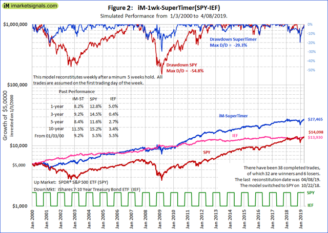(For those who are interested, the iM-1wk-SuperTimer with all the 15 component market timer models from its arsenal aroused would have produced $169,692, for an annualized return of 20.1% with a maximum drawdown of -10%. Thither would let been 45 completed trades, 39 of them winners.)

This clause was written by

Georg Vrba is a professional engineer WHO has been a consulting locomotive engineer for many years. In his opinion, mathematical models provide better steering to commercialise direction than financial "experts." He has developed financial models for the stock market, the draw together grocery store, yield kink, gold, silver and corne prediction, virtually of which are updated weekly at http://imarketsignals.com/.

Disclosure: I/we have no positions in any stocks mentioned, and no plans to initiate whatsoever positions within the next 72 hours. I wrote this article myself, and it expresses my own opinions. I am not receiving compensation for information technology. I experience no business human relationship with any company whose stock is mentioned in this article.